An Introduction to Dynamic Programming

Dynamic programming is a powerful technique used in computer science to solve complex problems efficiently. At its core, dynamic programming involves breaking down a problem into smaller subproblems, and then solving each subproblem only once. We can then combine the solutions to obtain the final result.

In this blog post, we’ll explore the basics of dynamic programming by starting with a simple ‘for’ loop and then moving on to recursive functions and how they can be substituted for this looping logic. We’ll use the Fibonacci sequence as an example to explain concepts such as BigO notation and memoization. By the end of this post, you’ll have a good understanding of dynamic programming and how it can be used to solve problems quickly and effectively.

Loops

Looping is a core part of programming and allows us to repeat a block of code many times without having to duplicate that code. Let’s look at a really simple for loop example:

function countdown(num: number) {
  for (let i = num; i >=0; i--) {
    console.log(i);
  }
}

If we were to run this function with countdown(10) then the output would be 10, 9, ..., 1, 0.

Recursive Functions

I’m sure the above doesn’t come as much surprise to you and that so far this is not a terribly exciting blog post, however, I am now going to duplicate this output by utilising a recursive function and not using a for while or do while loop:

function countdown(num: number) {
  if (num < 0) return;
  console.log(num);
  return countdown(num - 1)
}

If we run this function, the output would be exactly the same as the previous for loop example. So how does this work? Well, the function first of all has what we call a base case. A base case is crucial to prevent an situation where we start spawning an infinite number of countdown function execution contexts.

Execution Contexts and the Call Stack

Let’s rewind for a second and briefly explain what is meant by a function execution context. If you image a stack of plates in a kitchen then that is our call stack. At the bottom is our first ‘plate’ and it is our global execution context. This is created when we run our program. When we call a function then we create a new ‘plate’ and put it on the top of the stack. For JavaScript, the web browser or node server will only work on the top ‘plate’ however it can retain information and memory about the plates lower in the stack. Going back to our countdown example, we start by spawning a function execution context for the input 10 we check the base case and determine that it doesn't match the condition so we print 10 to the console. Next we call countdown again passing in 9 . This spawns a new function execution context and the same logic applies. It repeats this until the number is 0 which triggers the base case and that execution context is resolved. Once the execution context resolves, it is popped off the top of the stack. Check out this short demo inside Googles Chrome browser and pay attention to the call stack.

Video of the chrome browser call stack when execution a recursive function

OK, now that we are familiar with loops, the concept of recursion and the call stack, I want to show you something that you may have seen before but will now hopefully have a greater understanding of, the Fibonacci sequence recursive function! This function takes in a number and returns the value of the Fibonacci sequence at that index. For example if we input the number 7 it should return the value 21 as that is the value of the 7th number in the sequence. Note that this function uses 0 based indexing.

Let’s take a look at the source code for this recursive function:

const fib = (num: number) => {
  if (num === 0 || num === 1) return 1

  const res = fib(num - 1) + fib(num - 2)

  return res
}

Let’s break this down:

• The first line of the function is the base case that checks if num is equal to 0 or 1. If it is, then the function returns 1, because the first two numbers in the Fibonacci sequence are both 1.
• If num is not 0 or 1, then the function recursively calls itself twice, once with num - 1 and once with num - 2. These two calls represent calculating the two previous numbers in the Fibonacci sequence that are needed to calculate the current number.
• The results of these two recursive calls are added together and stored in the res variable.
• Finally, the res variable is returned, which represents the nth number in the Fibonacci sequence.

Let’s visualise this step by step by drawing out an inverse tree. We start at the top with the num being 5. Because this does not trigger the base case, we spawn a new function execution context where the new input num is equal to 4. We repeat this logic until we reach a function execution context on the top of the call stack where the num is equal to 1 or 0 and we return 1 . When we return, that function execution context is ‘popped’ off the top of the stack and that number is put in place of the fib(num -1) inside the function execution context that called the popped context. Once we reach the end of the ‘left’ side of the tree, we then start going to the right and we repeat the process as we move back up the tree, summing the numbers until we get to the top of the tree with the final sum.

A visual representation of the recursive function.

The above diagram shows the first function execution context having an input of 5 . As shown in parenthesis, the first call is to the left hand fib(num -1) that spawns its own context and it carries on that logic until the 18th step when it returns the number 5 as a response. The function execution contexts with a green border denote those that match the base case and immediately return the result of 1.

All in all, to calculate the 5th number of the sequence it took 28 steps not including the initial function call and return to the global execution context and the creation of 15 function execution contexts. This number will grow massively with every increment to the initial input number to the point where finding the 40th number could take a few seconds, but finding the 50th number could take minutes and anything above that causing your entire computer to lock up as it takes millions upon millions of steps!

Utilising Dynamic Programming

Let’s look at the diagram again. We can see that we are overlapping inputs and spawning new execution contexts. For example, we call fib(3) twice, and each time it spawns 4 additional contexts. We can optimise this by utilising memoization.

What this means is that when we treat each of these number inputs as its own subproblem. If we have not seen it before, then we calculate the result and then store that result in memory. Then if we see it again, we can immediately get the result from memory instead of re-calculating it again. In the above diagram this would mean at step 2 when we call fib(3) we would continue to calculate the result, but at step 19 when we call fib(3) again, we can immediately return 3 as we have the result stored in memory. We can do this for every number input and drastically cut down the number of steps needed to solve this problem. Calculating fib(50) can be reduced from millions upon millions of steps taking minutes to compute, to less than a hundred steps taking less than a millisecond.

Let’s alter our code to utilise memoization and the principle of dynamic programming:

const fib = (num: number, memo: Record<number, number> = {}) => {
  if (num === 0 || num === 1) return 1

  if (memo[num]) {
      return memo[num]
  }

  const res = fib(num - 1, memo) + fib(num - 2, memo)

  memo[num] = res  
  return res
}

We add a 2nd argument to the function called memo which is an object that acts as our memory store where the keys will be the index number and the value will be the Fibonacci number at that index. After the base case we look up the index number in the memo object and if it exists we return the value. This is hyper performant because looking up objects in this manner in JavaScript is O(1) or constant time. Check out Harvards CS50 for a primer on BigO notation if you are unfamiliar with it. But basically this means that the time it takes to retrieve the a value from the object given its key, will always be the same no matter how large the object grows.

Also because JavaScript passes objects by reference, that is it just passes around the address to the object in the computers memory rather than a copy of the object itself, the overhead is pretty much non existent.

The step by step flow of the improved function

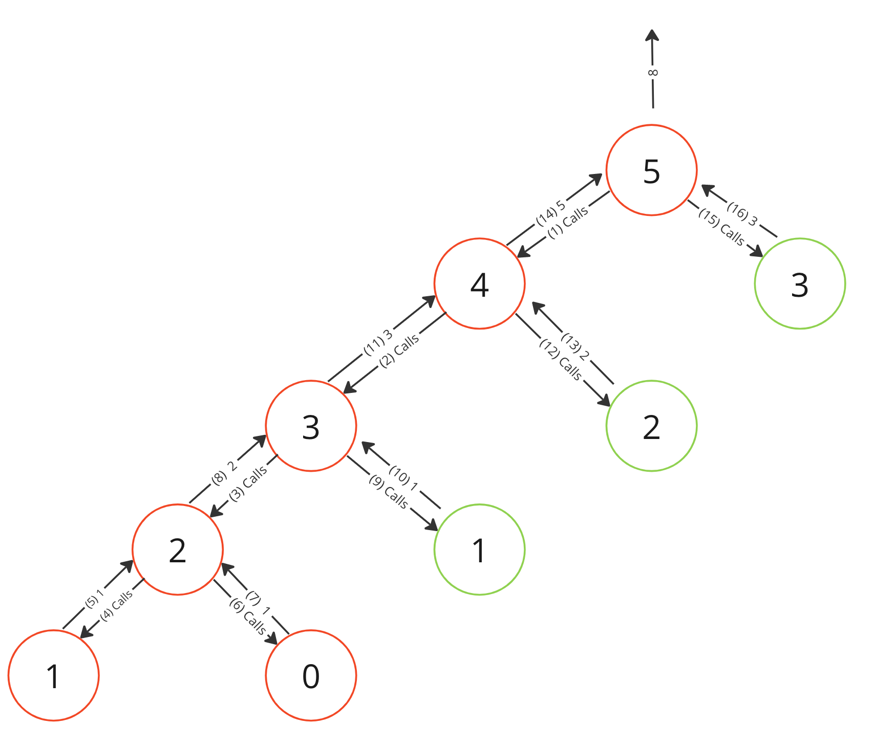
Looking at the new step-by-step flow, the function execution contexts in red are those that have an input that has not been memoized and so it spawns child function execution contexts to expensively calculate the result before storing that result and returning it to the parent function execution. The ones in green are those that do have an entry in the memo object and can immediately return the result without needed to do any additional work.

By utilising memoization, the time and space complexity of this program has gone from an exponential to linear which means as we increase the input number, instead of adding hundreds, thousands or millions+ more steps, we just add couple more each time the input increases.

A graph showing the number of function execution contexts created in our programs

Conclusion

In this blog post, we explored the basics of dynamic programming and how it can be used to solve complex problems efficiently. We started with a simple ‘for’ loop and then moved on to recursive functions and how they can be used to substitute looping logic. We used the Fibonacci sequence as an example to introduce concepts such as BigO notation and memoization. We also discussed execution contexts and the call stack in detail and how they are involved in the recursion process. Hopefully you should now have a solid understanding of dynamic programming and how it can be used to solve problems quickly and effectively. With this foundation, you can now explore more advanced techniques and apply dynamic programming to real-world problems.

Please check out my follow up article where we explore BigO notation in further detail and improve the performance of computing Fibonacci numbers even further!